t-plot calculations
Another common characterisation method is the t-plot method. First, make sure the data is imported by running the previous notebook.
[1]:
# import isotherms
%run import.ipynb

# import the characterisation module
import pygaps.characterisation as pgc
Selected 5 isotherms with nitrogen at 77K
Selected 2 room temperature calorimetry isotherms
Selected 2 isotherms for IAST calculation
Selected 3 isotherms for isosteric enthalpy calculation
Besides an isotherm, this method requires a so-called thickness function, which empirically describes the thickness of adsorbate layers on a non-porous surface as a function of pressure. It can be specified by the user, otherwise the "Harkins and Jura" thickness model is used by default. When the function is called without any other parameters, the framework will attempt to find plateaus in the data and automatically fit them with a straight line.
Let's look again at the our MCM-41 pore-controlled glass.
[2]:
isotherm = next(i for i in isotherms_n2_77k if i.material=='MCM-41')
print(isotherm.material)
results = pgc.t_plot(isotherm, verbose=True)
MCM-41
For linear region 1
The slope is 0.009732 and the intercept is 0.0002239, with a correlation coefficient of 1
The adsorbed volume is 0.00778 cm3/g and the area is 338.2 m2/g
For linear region 2
The slope is 0.001568 and the intercept is 0.008244, with a correlation coefficient of 0.9993
The adsorbed volume is 0.286 cm3/g and the area is 54.5 m2/g
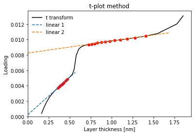
The first line can be attributed to adsorption on the inner pore surface, while the second one is adsorption on the external surface after pore filling. Two values are calculated for each section detected: the adsorbed volume and the specific area. In this case, the area of the first linear region corresponds to the pore area. Compare the specific surface area obtained of 340 \(m^2\) with the 360 \(m^2\) obtained through the BET method previously.
In the second region, the adsorbed volume corresponds to the total pore volume and the area is the external surface area of the sample.
We can get a better result for the surface area by attempting to have the first linear region at a zero intercept.
[3]:
print(isotherm.material)
results = pgc.t_plot(
    isotherm,
    thickness_model='Harkins/Jura',
    t_limits=(0.3,0.44),
    verbose=True
)
MCM-41
For linear region 1
The slope is 0.01003 and the intercept is 0.0001048, with a correlation coefficient of 0.9996
The adsorbed volume is 0.00364 cm3/g and the area is 348.4 m2/g
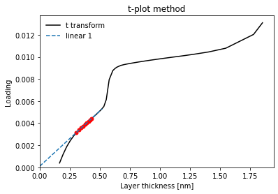
A near perfect match with the BET method. Of course, the method is only this accurate in certain cases, see more info in the documentation of the module. Let's do the calculations for all the nitrogen isotherms, using the same assumption that the first linear region is a good indicator of surface area.
[4]:
results = []
for isotherm in isotherms_n2_77k:
    results.append((isotherm.material, pgc.t_plot(isotherm, 'Harkins/Jura')))

[(x, f"{y['results'][0].get('area'):.2f}") for (x,y) in results]
[
    (<pygaps.Material 'MCM-41'>, '338.20'),
    (<pygaps.Material 'NaY'>, '199.77'),
    (<pygaps.Material 'SiO2'>, '249.14'),
    (<pygaps.Material 'Takeda 5A'>, '99.55'),
    (<pygaps.Material 'UiO-66(Zr)'>, '17.77')
]
We can see that, while we get reasonable values for the silica samples, all the rest are quite different. This is due to a number of factors depending on the material: adsorbate-adsorbent interactions having an effect on the thickness of the layer or simply having a different adsorption mechanism. The t-plot requires careful thought to assign meaning to the calculated values.
Since no thickness model can be universal, the framework allows for the thickness model to be substituted with an user-provided function which will be used for the thickness calculation, or even another isotherm, which will be converted into a thickness model.
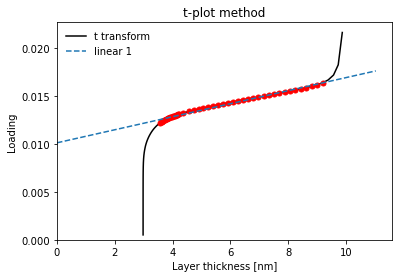
For example, using a carbon black type model:
[5]:
def carbon_model(relative_p):
    return 0.88*(relative_p**2) + 6.45*relative_p + 2.98

isotherm = next(i for i in isotherms_n2_77k if i.material=='Takeda 5A')
print(isotherm.material)
results = pgc.t_plot(isotherm, thickness_model=carbon_model, verbose=True)
Takeda 5A
For linear region 1
The slope is 0.0006789 and the intercept is 0.0101, with a correlation coefficient of 0.9939
The adsorbed volume is 0.351 cm3/g and the area is 23.59 m2/g
Isotherms which do not use nitrogen can also be used, but one should be careful that the thickness model is well chosen.
More information about the functions and their use can be found in the manual.