This page was generated from docs/examples/iast.ipynb. To start an interactive version:

IAST examples

The IAST method is used to predict the composition of the adsorbed phase in a multicomponent adsorption system, starting from pure component isotherms. First, make sure the data is imported by running the import notebook.

# import isotherms
%run import.ipynb

# import the iast module
import pygaps
import pygaps.iast as pgi

import matplotlib.pyplot as plt
import numpy

Selected 5 isotherms with nitrogen at 77K
Selected 2 room temperature calorimetry isotherms
Selected 2 isotherms for IAST calculation
Selected 3 isotherms for isosteric enthalpy calculation

Using models

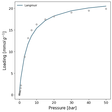
The IAST calculation is often performed by fitting a model to the isotherm rather than on the isotherms themselves, as spreading pressure can be computed efficiently when using most common models. Let's first fit the Langmuir model to both isotherms.

isotherms_iast_models = []

isotherm = next(i for i in isotherms_iast if i.material=='MOF-5(Zn)')
print('Isotherm sample:', isotherm.material)

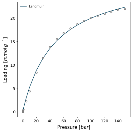
for isotherm in isotherms_iast:
    model = pygaps.ModelIsotherm.from_pointisotherm(isotherm, model='Langmuir', verbose=True)
    isotherms_iast_models.append(model)

Isotherm sample: MOF-5(Zn)
Attempting to model using Langmuir.
Model Langmuir success, RMSE is 0.901
Attempting to model using Langmuir.
Model Langmuir success, RMSE is 0.272

Now we can perform the IAST calculation with the resulting models. We specify the partial pressures of each component in the gaseous phase to obtain the composition of the adsorbed phase.

gas_fraction = [0.5, 0.5]
total_pressure = 10
pgi.iast_point_fraction(isotherms_iast_models, gas_fraction, total_pressure, verbose=True)

2 components.
        Partial pressure component 0 = 5
        Partial pressure component 1 = 5
Component 0
        p = 5
        p^0 = 5.71
        Loading = 11.01
        x = 0.8757
        Spreading pressure = 18.18
Component 1
        p = 5
        p^0 = 40.21
        Loading = 1.563
        x = 0.1243
        Spreading pressure = 18.18

array([11.0056369 ,  1.56267705])

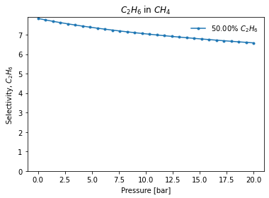
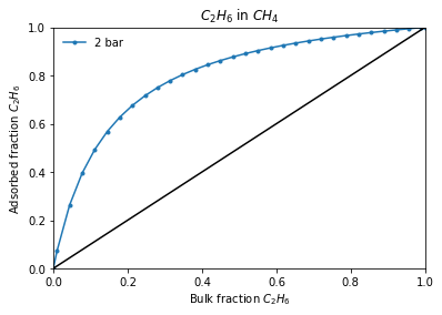
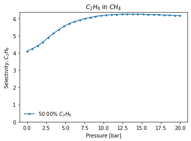
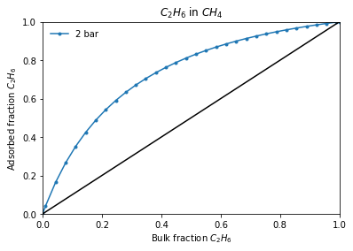
Alternatively, if we are interested in a binary system, we can use the extension functions iast_binary_svp and iast_binary_vle to obtain how the selectivity changes based on pressure in a constant composition or, respectively, how the gas phase-adsorbed phase changes with gas composition, at constant pressure.

These functions perform the IAST calculation at every point in the range passed and can plot the results. If interested in the selectivity for one component in an equimolar mixture over a pressure range:

mole_fractions = [0.5, 0.5]
pressure_range = numpy.linspace(0.01, 20, 30)

result_dict = pgi.iast_binary_svp(
    isotherms_iast_models,
    mole_fractions,
    pressure_range,
    verbose=True,
)

Or if interested on a adsorbed - gas phase equilibrium line:

total_pressure = 2
result_dict = pgi.iast_binary_vle(
    isotherms_iast_models,
    total_pressure,
    verbose=True,
)

Using isotherms directly - interpolation

The isotherms themselves can be used directly. However, instead of spreading pressure being calculated from the model, it will be approximated through interpolation and numerical quadrature integration.

gas_fraction = [0.5, 0.5]
total_pressure = 10
pgi.iast_point_fraction(
    isotherms_iast_models,
    gas_fraction,
    total_pressure,
    verbose=True,
)

2 components.
        Partial pressure component 0 = 5
        Partial pressure component 1 = 5
Component 0
        p = 5
        p^0 = 5.71
        Loading = 11.01
        x = 0.8757
        Spreading pressure = 18.18
Component 1
        p = 5
        p^0 = 40.21
        Loading = 1.563
        x = 0.1243
        Spreading pressure = 18.18

array([11.0056369 ,  1.56267705])

The binary mixture functions can also accept PointIsotherm objects.

mole_fraction = [0.5, 0.5]
pressure_range = numpy.linspace(0.01, 20, 30)

result_dict = pgi.iast_binary_svp(
    isotherms_iast,
    mole_fraction,
    pressure_range,
    verbose=True,
)

result_dict = pgi.iast_binary_vle(
    isotherms_iast,
    total_pressure=2,
    verbose=True,
)

More info about the method can be found in the manual.