This page was generated from docs/examples/dr_da_plots.ipynb. To start an interactive version:

Dubinin-Radushkevich and Dubinin-Astakov plots

The Dubinin-Radushkevich (DR) and Dubinin-Astakov (DA) plots are often used to determine the pore volume and the characteristic adsorption potential of adsorbent materials, in particular those of carbonaceous materials, such as activated carbons, carbon black or carbon nanotubes. It is also sometimes used for solution adsorption isotherms.

In pyGAPS, both the DR and DA plots are available with the dr_plot and da_plot functions. First we import the example isotherms.

# import isotherms
%run import.ipynb
%matplotlib inline

# import the characterisation module
import pygaps.characterisation as pgc

Selected 5 isotherms with nitrogen at 77K
Selected 2 room temperature calorimetry isotherms
Selected 2 isotherms for IAST calculation
Selected 3 isotherms for isosteric enthalpy calculation

Then we'll select the Takeda 5A isotherm to examine. We will perform a DR plot, with increased verbosity to observe the resulting linear fit. The function returns a dictionary with the calculated pore volume and adsorption potential.

isotherm = next(i for i in isotherms_n2_77k if i.material=='Takeda 5A')
results = pgc.dr_plot(isotherm, verbose=True)

Micropore volume is: 0.484 cm3/g
Effective adsorption potential is : 5.84 kJ/mol

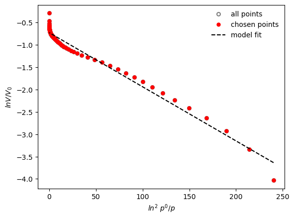
We can specify the pressure limits for the DR plot, to select only the points at low pressure for a better fit.

results = pgc.dr_plot(isotherm, p_limits=[0, 0.1], verbose=True)

Micropore volume is: 0.448 cm3/g
Effective adsorption potential is : 6 kJ/mol

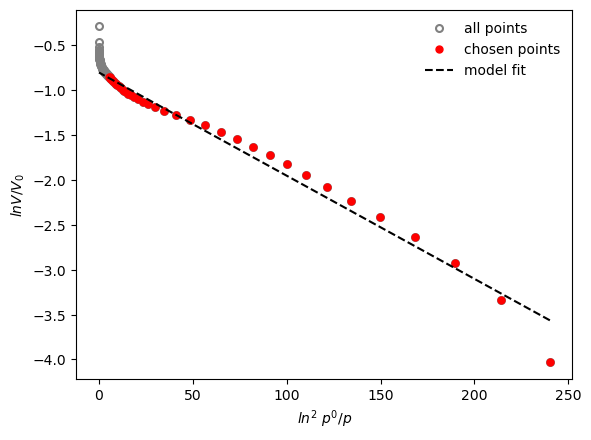
An extension of the DR model is the Dubinin-Astakov (DA) model. In the DA equation, the exponent can vary, and is usually chosen between 1 (for surfaces) and 3 (for micropores). For an explanation of the theory, check the function reference.

We then use the da_plot function and specify the exponent to be 2.3 (larger than the standard DR exponent of 2)

results = pgc.da_plot(isotherm, p_limits=[0,0.1], exp=2.3, verbose=True)

Micropore volume is: 0.422 cm3/g
Effective adsorption potential is : 6.34 kJ/mol

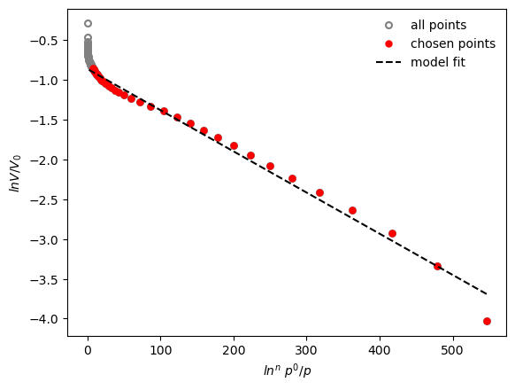
The DA plot can also automatically test which exponent gives the best fit between 1 and 3, if the parameter is left blank. The calculated exponent is returned in the result dictionary.

result = pgc.da_plot(isotherm, p_limits=[0, 0.1], exp=None, verbose=True)

Exponent is: 3
Micropore volume is: 0.385 cm3/g
Effective adsorption potential is : 6.92 kJ/mol

More info about the method can be found in the reference.