Specific surface area determination
BET surface area
Let's do a calculation of the BET area for these samples. First, make sure the data is imported by running the previous notebook.
[1]:
# import isotherms
%run import.ipynb

# import the characterisation module
import pygaps.characterisation as pgc
Selected 5 isotherms with nitrogen at 77K
Selected 2 room temperature calorimetry isotherms
Selected 2 isotherms for IAST calculation
Selected 3 isotherms for isosteric enthalpy calculation
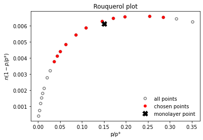
pyGAPS attempts to calculate the applicable BET region on its own by using the Rouquerol rules. The function is pygaps.characterisation.area_BET, where we set the verbose parameter to obtain a printed output of results and plots.
[2]:
isotherm = next(i for i in isotherms_n2_77k if i.material == 'MCM-41')
print(isotherm.material)
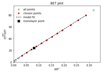
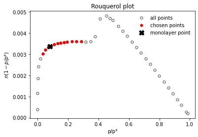
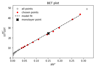
results = pgc.area_BET(isotherm, verbose=True)
MCM-41
BET area: a = 358.5 m2/g
The BET constant is: C = 129.2
Minimum pressure point is 0.0337 and maximum is 0.286
Statistical monolayer at: n = 0.00368 mol/g
The slope of the BET fit: s = 270
The intercept of the BET fit: i = 2.11
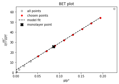
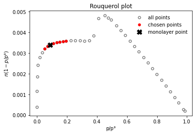
It looks that the correlation is reasonably good. A warning is emitted if this is not the case. We can also restrict the pressure range manually to see what difference it would make, by using the limits parameter.
[3]:
results = pgc.area_BET(isotherm, p_limits=(0.05, 0.2), verbose=True)
BET area: a = 361.7 m2/g
The BET constant is: C = 111.3
Minimum pressure point is 0.0513 and maximum is 0.194
Statistical monolayer at: n = 0.00371 mol/g
The slope of the BET fit: s = 267
The intercept of the BET fit: i = 2.42
Now let's do the analysis on all of the nitrogen samples. We'll assume the framework makes a reasonably accurate choice for the applicable range. The function returns a dictionary with all the calculated parameters, and we'll print the BET area from there.
[4]:
results = []
for isotherm in isotherms_n2_77k:
    results.append((isotherm.material, pgc.area_BET(isotherm)))

[(x, f"{y['area']:.2f}") for (x, y) in results]
[
    (<pygaps.Material 'MCM-41'>, '358.53'),
    (<pygaps.Material 'NaY'>, '699.23'),
    (<pygaps.Material 'SiO2'>, '210.39'),
    (<pygaps.Material 'Takeda 5A'>, '1109.80'),
    (<pygaps.Material 'UiO-66(Zr)'>, '1275.36')
]
We also have isotherms which were measured with \(CO_2\) at room temperature. While there's no guarantee that the BET method is still applicable with this adsorbate and temperature, we can still attempt to perform the calculations.
It just happens that the isotherms were recorded on the same Takeda 5A carbon sample (see \(N_2\) results above). Let's see how the \(CO_2\) BET surface area looks in comparison.
[5]:
isotherm = next(i for i in isotherms_calorimetry if i.material == 'Takeda 5A')
print(isotherm.material)
results = pgc.area_BET(isotherm, verbose=True)
Takeda 5A
BET area: a = 739.1 m2/g
The BET constant is: C = 31.7
Minimum pressure point is 0.0369 and maximum is 0.285
Statistical monolayer at: n = 0.00722 mol/g
The slope of the BET fit: s = 134
The intercept of the BET fit: i = 4.36
The surface area obtained with carbon dioxide is around 740 \(m^2\). Compared to the nitrogen surface area of 1100 \(m^2\), it is much smaller. While the checks implemented did not find anything wrong, this is likely due to interactions between carbon dioxide and the carbon surface leading to the breakdown of the BET theory.
While any kind of adsorbate and temperature (below critical) can be used, result interpretation is left at the discretion of the user. More info can be found in the documentation of the module.
Langmuir surface area
Another common method of calculating specific surface area relies on fitting the isotherm with a Langmuir model. This model assumes adsorption occurs on active surface/pore sites, in a single layer. We use the pygaps.characterisation.area_langmuir function, which defaults to a region of 0.1-0.9 p/p0 for the fitting (see documentation for details). We pass the verbose parameter to display the results automatically.
[6]:
isotherm = next(i for i in isotherms_n2_77k if i.material == 'MCM-41')
print(isotherm.material)
results = pgc.area_langmuir(isotherm, verbose=True)
MCM-41
The correlation is not linear.
Langmuir area: a = 1409 m2/g
Minimum pressure point is 0.0513 and maximum is 0.859
The Langmuir constant is: K = 2.72
Amount Langmuir monolayer is: n = 0.0144 mol/g
The slope of the Langmuir fit: s = 69.2
The intercept of the Langmuir fit: i = 25.4
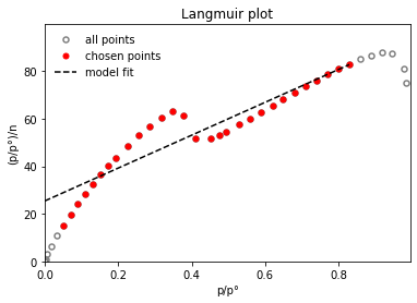
The correlation is not very good due to condensation in mesopores of MCM-41, which is not predicted by the Langmuir model. Due to this, the area calculated is not realistic. We can manually select a range in the monolayer adsorption regime for a better fit.
[7]:
print(isotherm.material)
results = pgc.area_langmuir(isotherm, p_limits=(0.05, 0.3), verbose=True)
MCM-41
Langmuir area: a = 550.1 m2/g
Minimum pressure point is 0.0513 and maximum is 0.286
The Langmuir constant is: K = 21.5
Amount Langmuir monolayer is: n = 0.00564 mol/g
The slope of the Langmuir fit: s = 177
The intercept of the Langmuir fit: i = 8.24
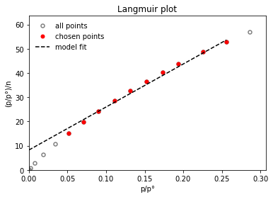
The fit is now better and the calculated area is also realistic. Comparing it to the BET area obtained previously, we see that it is higher by about 150 m2. Since adsorption is more likely to occur in monolayers until pore condensation, this method is not really suited for MCM-41. In general the Langmuir surface area is not as widely applicable as the BET one.
Now let's do the analysis on all of the nitrogen samples and compare the obtained surface areas with the BET ones.
[8]:
import matplotlib.pyplot as plt

area_langmuir = []
area_langmuir_lim = []
area_bet = []
for isotherm in isotherms_n2_77k:
    area_bet.append(pgc.area_BET(isotherm)['area'])
    area_langmuir.append(pgc.area_langmuir(isotherm)['area'])
    area_langmuir_lim.append(pgc.area_langmuir(isotherm, p_limits=(0.01, 0.3))['area'])

fig, (ax1, ax2) = plt.subplots(1, 2, figsize=(10, 5))
ax1.scatter(area_langmuir, area_bet)
ax2.scatter(area_langmuir_lim, area_bet)

ax1.set_title('BET v. Langmuir area, full range')
ax2.set_title('BET v. Langmuir area, LP range')

ax1.plot([0, 2000], [0, 2000], 'k--')
ax2.plot([0, 2000], [0, 2000], 'k--')

ax1.set_xlim(left=0, right=2000)
ax1.set_ylim(bottom=0, top=2000)
ax2.set_xlim(left=0, right=2000)
ax2.set_ylim(bottom=0, top=2000)

ax1.set_xlabel('Langmuir surface area [m2/g]')
ax1.set_ylabel('BET surface area [m2/g]')
ax2.set_xlabel('Langmuir surface area [m2/g]')
ax2.set_ylabel('BET surface area [m2/g]')
The correlation is not linear.
The correlation is not linear.
The correlation is not linear.
Text(0, 0.5, 'BET surface area [m2/g]')
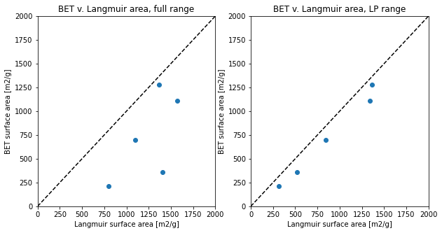
We can see that some points correspond, while others are not as well correlated. Unless the adsorption isotherm respects the Langmuir model, the calculated surface areas do not match. However, if the Langmuir area is calculated in a low pressure regime, ideally before multilayer adsorption or condensation occurs, the two specific areas are better correlated (right graph).
More info can be found in the documentation of the module.