The \(\alpha_s\) method
Very similar to the t-plot method, the \(\alpha_s\) method compares an isotherm on a porous material with one that was taken on a reference non-porous surface. The reference isotherm should be measured over a wide pressure range, to be able to compare loading values. First, make sure the data is imported notebook.
[1]:
# import isotherms
%run import.ipynb

# import the characterisation module
import pygaps.characterisation as pgc
Selected 5 isotherms with nitrogen at 77K
Selected 2 room temperature calorimetry isotherms
Selected 2 isotherms for IAST calculation
Selected 3 isotherms for isosteric enthalpy calculation
Unfortunately, we don't have a reference isotherm in our data. We are instead going to be creative and assume that the adsorption on the silica (\(SiO_2\) sample) is a good representation of an adsorption on a non-porous version of the MCM-41 sample. Let's try:
[2]:
iso_1 = next(i for i in isotherms_n2_77k if i.material == 'MCM-41')
iso_2 = next(i for i in isotherms_n2_77k if i.material == 'SiO2')

print(iso_1.material)
print(iso_2.material)
try:
    results = pgc.alpha_s(iso_1, reference_isotherm=iso_2, verbose=True)
except Exception as e:
    print('ERROR!:', e)
MCM-41
SiO2
ERROR!: A value in x_new is below the interpolation range.
The data in our reference isotherm is on a smaller range than that in the isotherm that we want to calculate! We are going to be creative again and first model the adsorption behaviour using a ModelIsotherm.
[3]:
import pygaps

model = pygaps.ModelIsotherm.from_pointisotherm(iso_2, model='BET', verbose=True)
Attempting to model using BET.
Model BET success, RMSE is 0.474
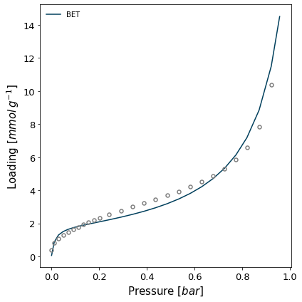
With our model fitting the data pretty well, we can now try the \(\alpha_s\) method again.
[4]:
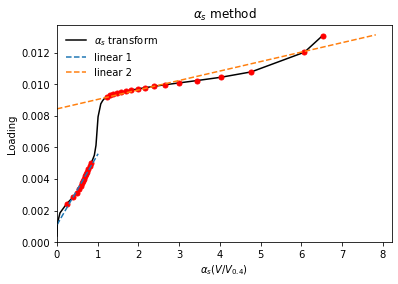
results = pgc.alpha_s(iso_1, model, verbose=True)
For linear region 0
The slope is 0.004462 and the intercept is 0.001096, with a correlation coefficient of 0.9848
The adsorbed volume is 0.0381 cm3/g and the area is 270.1 m2/g
For linear region 1
The slope is 0.0005994 and the intercept is 0.008443, with a correlation coefficient of 0.9656
The adsorbed volume is 0.293 cm3/g and the area is 36.28 m2/g
The results don't look that bad, considering all our assumptions and modelling. There are other parameters which can be specified for the \(\alpha_s\) function such as:
The relative pressure to use as the reducing pressure
The known area of the reference material. If this is not specified, the BET method is used to calculate the surface area.
As in the t-plot function, the limits for the straight line selection.
Read more about the theory in the documentation of the module and in the manual.