Quickstart
This document should get you started with pyGAPS, providing several common operations like creating/reading isotherms, running characterisation routines, model fitting and data export/plotting.
You can download this code as a Jupyter Notebook and run it for yourself! See banner at the top for the link.
Creating an isotherm
First, we need to import the package.
[1]:
%matplotlib inline
import pygaps as pg
The backbone of the framework is the PointIsotherm class. This class stores the isotherm data alongside isotherm properties such as the material, adsorbate and temperature, as well as providing easy interaction with the framework calculations. There are several ways to create a PointIsotherm object:
directly from arrays
from a
pandas.DataFrameparsing AIF, json, csv, or excel files
loading manufacturer reports (Micromeritics, Belsorp, 3P, Quantachrome, etc.)
loading from an sqlite database
See the isotherm creation part of the documentation for a more in-depth explanation. For the simplest method, the data can be passed in as arrays of pressure and loading. There are three other required metadata parameters: the adsorbent material name, the adsorbate molecule used, and the temperature at which the data was recorded.
[2]:
isotherm = pg.PointIsotherm(
    pressure=[0.1, 0.2, 0.3, 0.4, 0.5, 0.4, 0.35, 0.25, 0.15, 0.05],
    loading=[0.1, 0.2, 0.3, 0.4, 0.5, 0.45, 0.4, 0.3, 0.15, 0.05],
    material='Carbon X1',
    adsorbate='N2',
    temperature=77,
)
WARNING: 'pressure_mode' was not specified, assumed as 'absolute'
WARNING: 'pressure_unit' was not specified, assumed as 'bar'
WARNING: 'material_basis' was not specified, assumed as 'mass'
WARNING: 'material_unit' was not specified, assumed as 'g'
WARNING: 'loading_basis' was not specified, assumed as 'molar'
WARNING: 'loading_unit' was not specified, assumed as 'mmol'
WARNING: 'temperature_unit' was not specified, assumed as 'K'
We can see that most units are set to defaults and we are being notified about it. Let's assume we don't want to change anything for now.
To see a summary of the isotherm metadata, use the print function:
[3]:
print(isotherm)
Material: Carbon X1
Adsorbate: nitrogen
Temperature: 77.0K
Units:
        Uptake in: mmol/g
        Pressure in: bar
Unless specified, the loading is read in mmol/g and the pressure is read in bar. We can specify (and convert) units to anything from weight% vs Pa, mol/cm3 vs relative pressure to cm3/mol vs torr. Read more about how pyGAPS handles units in this section of the manual. The isotherm can also have other properties which are passed in at creation.
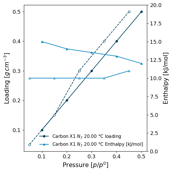
Alternatively, the data can be passed in the form of a pandas.DataFrame. This allows for other complementary data, such as ambient pressure, isosteric enthalpy, or other simultaneous measurements corresponding to each point to be saved.
The DataFrame should have at least two columns: the pressures at which each point was recorded, and the loadings for each point. The loading_key and pressure_key parameters specify which column in the DataFrame contain the loading and pressure, respectively. We will also take the opportunity to set our own units, and a few extra metadata properties.
[4]:
import pandas as pd

# create (or import) a DataFrame
data = pd.DataFrame({
    'pressure': [0.1, 0.2, 0.3, 0.4, 0.5, 0.45, 0.35, 0.25, 0.15, 0.05],
    'loading': [0.1, 0.2, 0.3, 0.4, 0.5, 0.5, 0.4, 0.3, 0.15, 0.05],
    'Enthalpy [kJ/mol]': [15, 14, 13.5, 13, 12, 11, 10, 10, 10, 10],
})

isotherm = pg.PointIsotherm(
    isotherm_data=data,
    pressure_key='pressure',
    loading_key='loading',

    material='Carbon X1',
    adsorbate='N2',
    temperature=20,

    pressure_mode='relative',
    pressure_unit=None,  # we are in relative mode
    loading_basis='mass',
    loading_unit='g',
    material_basis='volume',
    material_unit='cm3',
    temperature_unit='°C',

    material_batch='Batch 1',
    iso_type='characterisation'
)
All passed metadata is stored in the isotherm.properties dictionary.
[5]:
print(isotherm.properties)
{'material_batch': 'Batch 1', 'iso_type': 'characterisation'}
A summary and a plot can be generated by using the print_info function. Notice how the units are automatically taken into account in the plots.
[6]:
isotherm.print_info(y2_range=[0, 20])
Material: Carbon X1
Adsorbate: nitrogen
Temperature: 293.15K
Units:
        Uptake in: g/cm3
        Relative pressure
Other properties:
        material_batch: Batch 1
        iso_type: characterisation
(
    <AxesSubplot:xlabel='Pressure [$p/p^0$]', ylabel='Loading [$g\\/cm^{-3}$]'>,
    <AxesSubplot:ylabel='Enthalpy [kJ/mol]'>
)
pyGAPS also comes with a variety of parsers that allow isotherms to be saved or loaded. Here we can use the JSON parser to get an isotherm previously saved on disk. For more info on parsing to and from various formats see the manual and the associated examples.
[7]:
import pygaps.parsing as pgp
isotherm = pgp.isotherm_from_json(r'data/carbon_x1_n2.json')
We can then inspect the isotherm data using various functions:
[8]:
isotherm.data()
[8]:
| pressure | loading | branch | |
|---|---|---|---|
| 0 | 1.884754e-07 | 0.510281 | 0 |
| 1 | 4.498150e-07 | 1.022560 | 0 |
| 2 | 1.058960e-06 | 1.541660 | 0 |
| 3 | 2.360800e-06 | 2.059750 | 0 |
| 4 | 4.935335e-06 | 2.580030 | 0 |
| ... | ... | ... | ... |
| 126 | 1.717322e-01 | 12.969600 | 1 |
| 127 | 1.478162e-01 | 12.792700 | 1 |
| 128 | 1.243666e-01 | 12.582000 | 1 |
| 129 | 1.028454e-01 | 12.337100 | 1 |
| 130 | 8.843120e-02 | 12.138200 | 1 |
131 rows × 3 columns
[9]:
isotherm.pressure(branch="des")
array([0.94224978, 0.9175527 , 0.88026274, 0.85005033, 0.8250035 ,
       0.79809718, 0.75394244, 0.72825927, 0.70260524, 0.67857171,
       0.65424575, 0.63045607, 0.60668388, 0.58312446, 0.55678356,
       0.53354765, 0.50847557, 0.48454113, 0.46082723, 0.4361253 ,
       0.41206068, 0.38803881, 0.36445995, 0.33972693, 0.3160004 ,
       0.29139658, 0.26721247, 0.24362584, 0.21954373, 0.195449  ,
       0.17173219, 0.14781621, 0.12436657, 0.1028454 , 0.0884312 ])
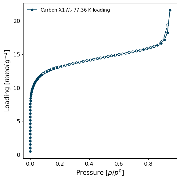
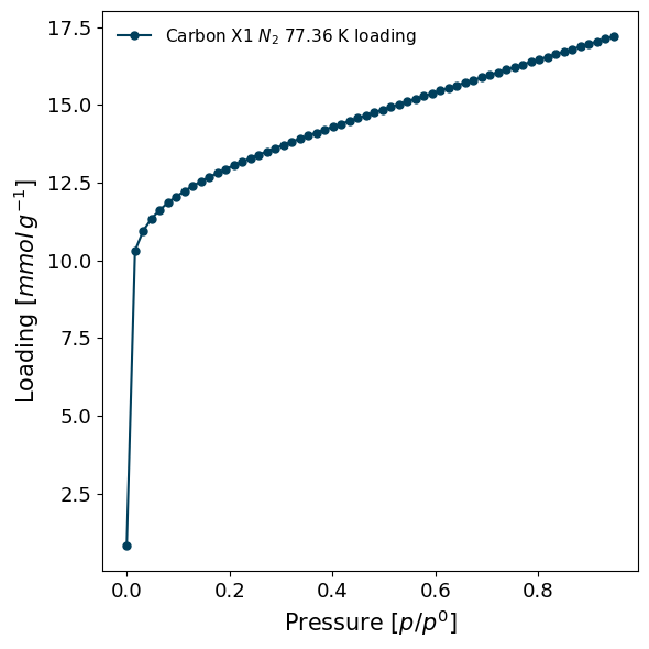
To see just a plot of the isotherm, use the plot function:
[10]:
isotherm.plot()

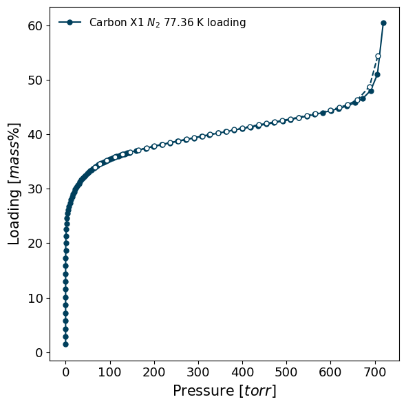
Isotherms can be plotted in different units/modes, or can be permanently converted. If conversion is desired, find out more in this section. For example, using the previous isotherm:
[11]:
# This just displays the isotherm in a different unit
isotherm.plot(pressure_unit='torr', loading_basis='percent')
# The isotherm is still internally in the same units
print(f"Isotherm is still in {isotherm.pressure_unit} and {isotherm.loading_unit}.")
Isotherm is still in bar and mmol.
[12]:
# While the underlying units can be completely converted
isotherm.convert(pressure_mode='relative')
print(f"Isotherm is now permanently in {isotherm.pressure_mode} pressure.")
isotherm.plot()
Isotherm is now permanently in relative pressure.
Now that the PointIsotherm is created, we are ready to do some analysis of its properties.
Isotherm analysis
The framework has several isotherm analysis tools which are commonly used to characterise porous materials such as:
BET surface area
the t-plot method / alpha s method
mesoporous PSD (pore size distribution) calculations
microporous PSD calculations
DFT kernel fitting PSD methods
isosteric enthalpy of adsorption calculation
and much more...
All methods work directly with generated Isotherms. For example, to perform a t-plot analysis and get the results in a dictionary use:
[13]:
import pprint
import pygaps.characterisation as pgc

result_dict = pgc.t_plot(isotherm)
pprint.pprint(result_dict)
{'results': [{'adsorbed_volume': 0.06225102073354812,
              'area': 1033.1609271782331,
              'corr_coef': 0.9998068073094798,
              'intercept': 1.7912656114940457,
              'section': [22, 23, 24, 25, 26, 27, 28, 29],
              'slope': 29.72908103651894},
             {'adsorbed_volume': 0.410455160252538,
              'area': 139.1041773312518,
              'corr_coef': 0.9836601580118213,
              'intercept': 11.81079771796286,
              'section': [64,
                          65,
                          66,
                          67,
                          68,
                          69,
                          70,
                          71,
                          72,
                          73,
                          74,
                          75,
                          76,
                          77,
                          78,
                          79,
                          80,
                          81,
                          82,
                          83,
                          84,
                          85,
                          86,
                          87,
                          88,
                          89,
                          90,
                          91,
                          92],
              'slope': 4.002705920842157}],
 't_curve': array([0.14381104, 0.14800322, 0.1525095 , 0.15712503, 0.1617626 ,
       0.16612841, 0.17033488, 0.17458578, 0.17879119, 0.18306956,
       0.18764848, 0.19283516, 0.19881473, 0.2058225 , 0.21395749,
       0.2228623 , 0.23213447, 0.2411563 , 0.24949659, 0.25634201,
       0.2635719 , 0.27002947, 0.27633547, 0.28229453, 0.28784398,
       0.29315681, 0.29819119, 0.30301872, 0.30762151, 0.31210773,
       0.31641915, 0.32068381, 0.32481658, 0.32886821, 0.33277497,
       0.33761078, 0.34138501, 0.34505614, 0.34870159, 0.35228919,
       0.35587619, 0.35917214, 0.36264598, 0.36618179, 0.36956969,
       0.37295932, 0.37630582, 0.37957513, 0.38277985, 0.38608229,
       0.3892784 , 0.3924393 , 0.39566979, 0.39876923, 0.40194987,
       0.40514492, 0.40824114, 0.41138787, 0.41450379, 0.41759906,
       0.42072338, 0.42387825, 0.42691471, 0.43000525, 0.44357547,
       0.46150731, 0.47647445, 0.49286816, 0.50812087, 0.52341251,
       0.53937129, 0.55659203, 0.57281485, 0.5897311 , 0.609567  ,
       0.62665975, 0.64822743, 0.66907008, 0.69046915, 0.71246898,
       0.73767931, 0.76126425, 0.79092372, 0.82052677, 0.85273827,
       0.88701466, 0.92485731, 0.96660227, 1.01333614, 1.06514197,
       1.1237298 , 1.19133932, 1.27032012, 1.36103511, 1.45572245,
       1.55317729])}
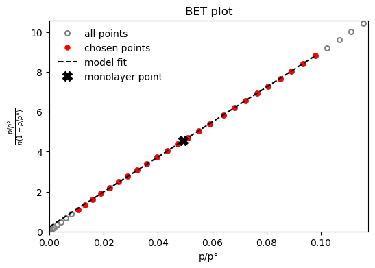
If in an interactive environment, such as iPython or Jupyter, it is useful to see the details of the calculation directly. To do this, increase the verbosity of the method to display extra information, including graphs:
[14]:
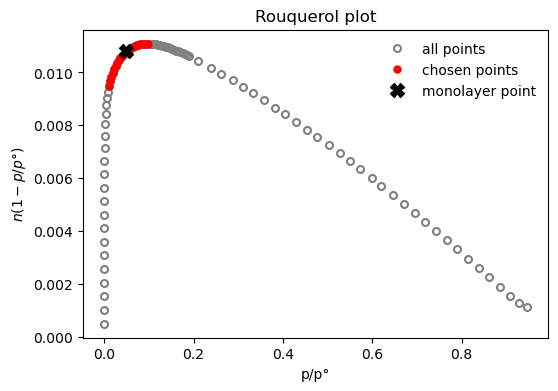
result_dict = pgc.area_BET(isotherm, verbose=True)
BET area: a = 1110 m2/g
The BET constant is: C = 372.8
Minimum pressure point is 0.0105 and maximum is 0.0979
Statistical monolayer at: n = 0.0114 mol/g
The slope of the BET fit: s = 87.7
The intercept of the BET fit: i = 0.236
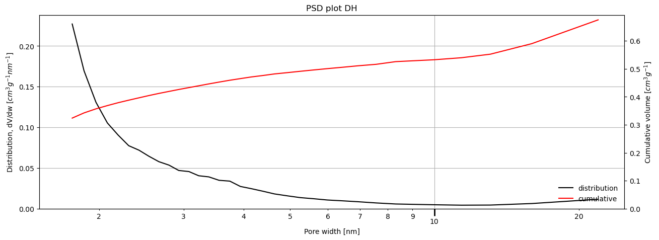
Depending on the method, parameters can be specified to tweak the way the calculations are performed. For example, if a mesoporous size distribution is desired using the Dollimore-Heal method on the desorption branch of the isotherm, assuming the pores are cylindrical and that adsorbate thickness can be described by a Halsey-type thickness curve, the code will look like:
[15]:
result_dict = pgc.psd_mesoporous(
    isotherm,
    psd_model='DH',
    branch='des',
    pore_geometry='cylinder',
    thickness_model='Halsey',
    verbose=True,
)
For more information on how to use each method, check the manual and the associated examples.
Isotherm fitting
The framework comes with functionality to fit point isotherm data with common isotherm models such as Henry, Langmuir, Temkin, Virial etc.
The model is contained in the ModelIsotherm class. The class is similar to the PointIsotherm class, and shares the parameters and metadata. However, instead of point data, it stores model coefficients for the model it's describing.
To create a ModelIsotherm, the same parameters dictionary / pandas.DataFrame procedure can be used. But, assuming we've already created a PointIsotherm object, we can just pass it to the pygaps.model_iso function.
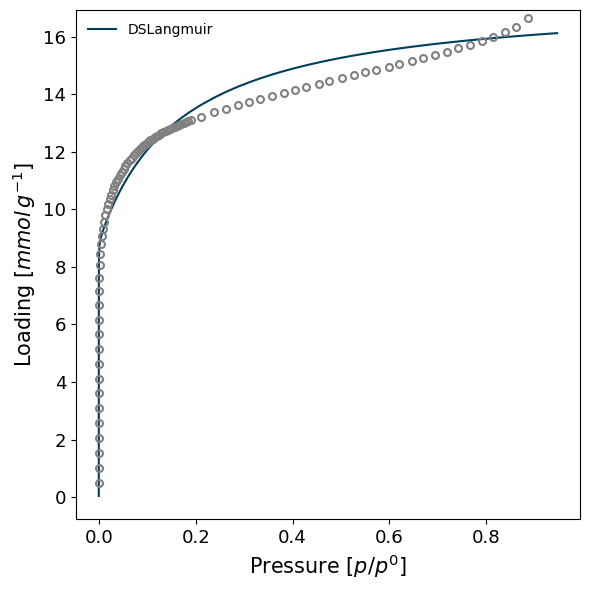
[16]:
import pygaps.modelling as pgm

model_iso = pgm.model_iso(isotherm, model='DSLangmuir', verbose=True)
model_iso
Attempting to model using DSLangmuir.
Model DSLangmuir success, RMSE is 0.0402
<ModelIsotherm 38c2a31aae475e0e5f6285194152baf0>: 'nitrogen' on 'Carbon X1' at 77.355 K
A minimisation procedure will then attempt to fit the model's parameters to the isotherm points. If successful, the ModelIsotherm is returned.
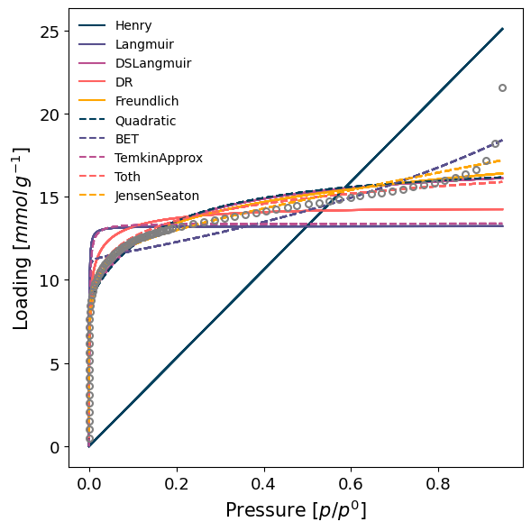
In the user wants to screen several models at once, the model can be given as guess, to try to find the best fitting model. Below, we will attempt to fit several simple available models, and the one with the best RMSE will be returned. This method may take significant processing time, and there is no guarantee that the model is physically relevant.
[17]:
model_iso = pgm.model_iso(isotherm, model='guess', verbose=True)
Attempting to model using Henry.
Model Henry success, RMSE is 0.352
Attempting to model using Langmuir.
Model Langmuir success, RMSE is 0.101
Attempting to model using DSLangmuir.
Model DSLangmuir success, RMSE is 0.0402
Attempting to model using DR.
Model DR success, RMSE is 0.0623
Attempting to model using Freundlich.
Model Freundlich success, RMSE is 0.035
Attempting to model using Quadratic.
Model Quadratic success, RMSE is 0.0402
Attempting to model using BET.
Model BET success, RMSE is 0.0515
Attempting to model using TemkinApprox.
Model TemkinApprox success, RMSE is 0.0971
Attempting to model using Toth.
Model Toth success, RMSE is 0.0358
Attempting to model using JensenSeaton.
Model JensenSeaton success, RMSE is 0.0253
Best model fit is JensenSeaton.
More advanced settings can also be specified, such as the parameters for the fitting routine or the initial parameter guess. For in-depth examples and discussion check the manual and the associated examples.
To print the model parameters use the same print method as before.
[18]:
# Prints isotherm parameters and model info
model_iso.print_info()
Material: Carbon X1
Adsorbate: nitrogen
Temperature: 77.355K
Units:
        Uptake in: mmol/g
        Relative pressure
Other properties:
        plot_fit: False
        material_batch: X1
        iso_type: physisorption
        user: PI
        instrument: homemade1
        activation_temperature: 150.0
        lab: local
        treatment: acid activated
JensenSeaton isotherm model.
RMSE = 0.02527
Model parameters:
        K = 5.516e+08
        a = 16.73
        b = 0.3403
        c = 0.1807
Model applicable range:
        Pressure range: 1.86e-07 - 0.946
        Loading range: 0.51 - 21.6
We can calculate the loading at any pressure using the internal model by using the loading_at function.
[19]:
# Returns the loading at 1 bar calculated with the model
model_iso.loading_at(1.0)
17.46787643653736
[20]:
# Returns the loading for three points in the 0-1 bar range
pressure = [0.1,0.5,1]
model_iso.loading_at(pressure)
array([12.09708239, 14.86182185, 17.46787644])
Plotting
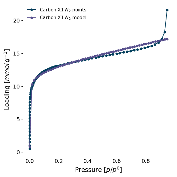
pyGAPS makes graphing both PointIsotherm and ModelIsotherm objects easy to facilitate visual observations, inclusion in publications and consistency. Plotting an isotherm is as simple as:
[21]:
import pygaps.graphing as pgg

pgg.plot_iso(
    [isotherm, model_iso],                          # Two isotherms
    branch='ads',                                   # Plot only the adsorption branch
    lgd_keys=['material', 'adsorbate', 'type'],     # Text in the legend, as taken from the isotherms
)
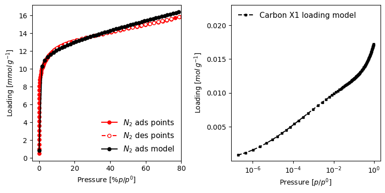
Here is a more involved plot, where we create the figure beforehand, and specify many more customisation options.
[22]:
import matplotlib.pyplot as plt

fig, (ax1, ax2) = plt.subplots(1, 2, figsize=(8, 4))

pgg.plot_iso(
    [isotherm, model_iso],
    ax=ax1,
    branch='all',
    pressure_mode="relative%",
    x_range=(None, 80),
    color=["r", "k"],
    lgd_keys=['adsorbate', 'branch', 'type'],
)

model_iso.plot(
    ax=ax2,
    x_points=isotherm.pressure(),
    loading_unit="mol",
    y1_range=(None, 0.023),
    marker="s",
    color="k",
    y1_line_style={
        "linestyle": "--",
        "markersize": 3
    },
    logx=True,
    lgd_pos="upper left",
    lgd_keys=['material', 'key', 'type'],
)
Many settings can be specified to change the look and feel of the graphs. More explanations can be found in the manual and in the examples section.